Pareto front

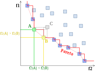
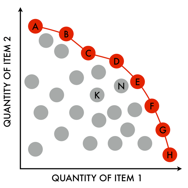
In multi-objective optimization, the Pareto front (also called Pareto frontier or Pareto curve) is the set of all Pareto efficient solutions.^[1] The concept is widely used in engineering.^{[2]: 111–148} It allows the designer to restrict attention to the set of efficient choices, and to make tradeoffs within this set, rather than considering the full range of every parameter.^{[3]: 63–65 [4]: 399–412}

Example of a Pareto frontier. The boxed points represent feasible choices, and smaller values are preferred to larger ones. Point C is not on the Pareto frontier because it is dominated by both point A and point B. Points A and B are not strictly dominated by any other, and hence lie on the frontier.

A production-possibility frontier. The red line is an example of a Pareto-efficient frontier, where the frontier and the area left and below it are a continuous set of choices. The red points on the frontier are examples of Pareto-optimal choices of production. Points off the frontier, such as N and K, are not Pareto-efficient, since there exist points on the frontier which Pareto-dominate them.

Definition

The Pareto frontier, P(Y), may be more formally described as follows. Consider a system with function ${\displaystyle f:X\rightarrow \mathbb {R} ^{m}}$, where X is a compact set of feasible decisions in the metric space ${\displaystyle \mathbb {R} ^{n}}$, and Y is the feasible set of criterion vectors in ${\displaystyle \mathbb {R} ^{m}}$, such that ${\displaystyle Y=\{y\in \mathbb {R} ^{m}:\;y=f(x),x\in X\;\}}$.

We assume that the preferred directions of criteria values are known. A point ${\displaystyle y^{\prime \prime }\in \mathbb {R} ^{m}}$ is preferred to (strictly dominates) another point ${\displaystyle y^{\prime }\in \mathbb {R} ^{m}}$, written as ${\displaystyle y^{\prime \prime }\succ y^{\prime }}$. The Pareto frontier is thus written as:

${\displaystyle P(Y)=\{y^{\prime }\in Y:\;\{y^{\prime \prime }\in Y:\;y^{\prime \prime }\succ y^{\prime },y^{\prime }\neq y^{\prime \prime }\;\}=\emptyset \}.}$

Marginal rate of substitution

A significant aspect of the Pareto frontier in economics is that, at a Pareto-efficient allocation, the marginal rate of substitution is the same for all consumers.^[5] A formal statement can be derived by considering a system with m consumers and n goods, and a utility function of each consumer as ${\displaystyle z_{i}=f^{i}(x^{i})}$ where ${\displaystyle x^{i}=(x_{1}^{i},x_{2}^{i},\ldots ,x_{n}^{i})}$ is the vector of goods, both for all i. The feasibility constraint is ${\displaystyle \sum _{i=1}^{m}x_{j}^{i}=b_{j}}$ for ${\displaystyle j=1,\ldots ,n}$. To find the Pareto optimal allocation, we maximize the Lagrangian:

${\displaystyle L_{i}((x_{j}^{k})_{k,j},(\lambda _{k})_{k},(\mu _{j})_{j})=f^{i}(x^{i})+\sum _{k=2}^{m}\lambda _{k}(z_{k}-f^{k}(x^{k}))+\sum _{j=1}^{n}\mu _{j}\left(b_{j}-\sum _{k=1}^{m}x_{j}^{k}\right)}$

where ${\displaystyle (\lambda _{k})_{k}}$ and ${\displaystyle (\mu _{j})_{j}}$ are the vectors of multipliers. Taking the partial derivative of the Lagrangian with respect to each good ${\displaystyle x_{j}^{k}}$ for ${\displaystyle j=1,\ldots ,n}$ and ${\displaystyle k=1,\ldots ,m}$ gives the following system of first-order conditions:

${\displaystyle {\frac {\partial L_{i}}{\partial x_{j}^{i}}}=f_{x_{j}^{i}}^{1}-\mu _{j}=0{\text{ for }}j=1,\ldots ,n,}$

${\displaystyle {\frac {\partial L_{i}}{\partial x_{j}^{k}}}=-\lambda _{k}f_{x_{j}^{k}}^{i}-\mu _{j}=0{\text{ for }}k=2,\ldots ,m{\text{ and }}j=1,\ldots ,n,}$

where ${\displaystyle f_{x_{j}^{i}}}$ denotes the partial derivative of ${\displaystyle f}$ with respect to ${\displaystyle x_{j}^{i}}$. Now, fix any ${\displaystyle k\neq i}$ and ${\displaystyle j,s\in \{1,\ldots ,n\}}$. The above first-order condition imply that

${\displaystyle {\frac {f_{x_{j}^{i}}^{i}}{f_{x_{s}^{i}}^{i}}}={\frac {\mu _{j}}{\mu _{s}}}={\frac {f_{x_{j}^{k}}^{k}}{f_{x_{s}^{k}}^{k}}}.}$

Thus, in a Pareto-optimal allocation, the marginal rate of substitution must be the same for all consumers.^{[citation needed]}

Computation

Algorithms for computing the Pareto frontier of a finite set of alternatives have been studied in computer science and power engineering.^[6] They include:

• "The maxima of a point set"
• "The maximum vector problem" or the skyline query^[7][8][9]
• "The scalarization algorithm" or the method of weighted sums^[10][11]
• "The ${\displaystyle \epsilon }$-constraints method"^[12][13][14]
• Multi-objective Evolutionary Algorithms ^[15][16]

Approximations

Since generating the entire Pareto front is often computationally-hard, there are algorithms for computing an approximate Pareto-front. For example, Legriel et al.^[17] call a set S an ε-approximation of the Pareto-front P, if the directed Hausdorff distance between S and P is at most ε. They observe that an ε-approximation of any Pareto front P in d dimensions can be found using (1/ε)^d queries.

Zitzler, Knowles and Thiele^[18] compare several algorithms for Pareto-set approximations on various criteria, such as invariance to scaling, monotonicity, and computational complexity.