Mosaic plot

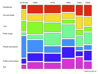
A mosaic plot, Marimekko chart, Mekko chart, or sometimes percent stacked bar plot, is a graphical visualization of data from two or more qualitative variables.^[1] It is the multidimensional extension of spineplots, which graphically display the same information for only one variable.^[2] It gives an overview of the data and makes it possible to recognize relationships between different variables. For example, independence is shown when the boxes across categories all have the same areas.^[3] Mosaic plots were introduced by Hartigan and Kleiner in 1981 and expanded on by Friendly in 1994.^{[4] [5]} Mosaic plots are also called Marimekko or Mekko charts because they resemble some Marimekko prints.^[6][7] However, in statistical applications, mosaic plots can be colored and shaded according to deviations from independence, whereas Marimekko charts are colored according to the category levels, as in the image.

Mosaic plot showing cross-sectional distribution through time of different musical themes in the Guardian's list of "1000 songs to hear before you die".

As with bar charts and spineplots, the area of the tiles, also known as the bin size, is proportional to the number of observations within that category.^[8]

Example

An example of mosaic plots uses data from the passengers on the Titanic. There are 2201 observations and 3 variables. The variables are:

• the gender of the person (male / female)
• the class (1st, 2nd and 3rd class, or crew)
• did this person survive the sinking (yes / no)?

Gender	Survived	1st Class	2nd Class	3rd Class	Crew
Male	No	118	154	422	670
	Yes	62	25	88	192
Female	No	4	13	106	3
	Yes	141	93	90	20

Mosaic plot construction

Order	Variable	Axis
1.	Gender	Vertical
2.	Class	Horizontal
3.	Survived	Vertical

The categorical variables are first put in order. Then, each variable is assigned to an axis. In the table to the right, sequence and classification is presented for this data set. Another ordering will result in a different mosaic plot, i.e., the order of the variables is significant as for all multivariate plots.

At the left edge of the first variable we first plot "Gender," meaning that we divide the data vertically in two blocks: the bottom blocks corresponds to females, while the upper (much larger) one to males. One immediately sees that roughly a quarter of the passengers were female and the remaining three quarters male.

One then applies the second variable "Class" to the top edge. The four vertical columns therefore mark the four values of that variable (1st, 2nd, 3rd, and crew). These columns are of variable thickness, because column width indicates the relative proportion of the corresponding value on the population. Crew plainly represents the largest male group, whereas third-class passengers are the largest female group. The number of female crew members is also seen to have been marginal.

The last variable ("Survived") is finally applied, this time along the left edge with the result highlighted by shade: dark grey rectangles represent people that did not survive the disaster, light grey ones people that did. Women in the first class are immediately seen to have had the highest survival probability. The survival probability for females is seen to have been higher than that for men (marginalised over all classes). Similarly, a marginalization over gender identifies first-class passengers as most probable to survive. Overall, about 1/3 of all people survived (proportion of light gray areas).

Properties

• The displayed variables are categorical or ordinal scales.
• The plot is of at least two variables. There is no upper limit, but too many variables may be confusing in graphic form.
• The number of observations is not limited, but not read in the image.
• The areas of the rectangular tiles that are available for a combination of features are proportional to the number of observations that have this combination of features.
• Unlike, for example, the boxplot or QQ plot, it is not possible for the mosaic plot to plot a confidence interval. However, the tiles can be colored according to the standardized residual from a model of independence, so that cells with excessively large or small deviations are shaded to show those that are 'significant' and the pattern of association can be discerned.

Criticism

The mosaic plot has been criticised for making the data hard to perceive and to compare visually, because the values correspond to areas.^[9][7]

See also

• Heat map
• Treemap
• Contingency table

References

1. Sandra D. Schlotzhauer (1 April 2007). Elementary Statistics Using JMP. SAS Institute. p. 407. ISBN 978-1-59994-428-9.
2. New Techniques and Technologies for Statistics II: Proceedings of the Second Bonn Seminar. IOS Press. 1 January 1997. p. 254. ISBN 978-90-5199-326-4.
3. Michael Friendly (1 January 1991). SAS System for Statistical Graphics. SAS Institute. pp. 512–. ISBN 978-1-55544-441-9.
4. SAS Institute (6 September 2013). JMP 11 Basic Analysis. SAS Institute. pp. 251–. ISBN 978-1-61290-684-3.
5. Michael Friendly & David Meyer (2016). Discrete Data Analysis with R: Visualization and Modeling Techniques for Categorical and Count Data. Chapman & Hall/CRC. ISBN 978-1-4987-2583-5.
6. Smith, Alan (6 September 2017). "How to apply Marimekko to data". Financial Times. Retrieved 27 September 2019.
7. "Marimekko Chart". Mekko Graphics. Retrieved 13 December 2017.
8. Martin Theus; Simon Urbanek (23 March 2011). Interactive Graphics for Data Analysis: Principles and Examples. CRC Press. ISBN 978-1-4200-1106-7.
9. Few, Stephen. "Design Example: Marimekko Chart". Perceptual Edge. Retrieved 30 October 2011.

Further reading

• John Hartigan, Beat Kleiner: Mosaics for contingency tables. In: Computer Science and Statistics: Proceedings of the 13th Symposium on the Interface. 1981, S. 268–273.
• Michael Friendly: A Brief History of the Mosaic Display In: Journal of Computational and Graphical Statistics, 2002, 11, 89–107. [The earliest known mosaic display goes back to Georg von Mayr (1877).]