Rank–size distribution

Rank–size distribution is the distribution of size by rank, in decreasing order of size. For example, if a data set consists of items of sizes 5, 100, 5, and 8, the rank-size distribution is 100, 8, 5, 5 (ranks 1 through 4). This is also known as the rank–frequency distribution, when the source data are from a frequency distribution. These are particularly of interest when the data vary significantly in scales, such as city size or word frequency. These distributions frequently follow a power law distribution, or less well-known ones such as a stretched exponential function or parabolic fractal distribution, at least approximately for certain ranges of ranks; see below.

Rank–size distribution of the population of countries follows a stretched exponential distribution^[1] except in the cases of the two "Kings": China and India.

A rank-size distribution is not a probability distribution or cumulative distribution function. Rather, it is a discrete form of a quantile function (inverse cumulative distribution) in reverse order, giving the size of the element at a given rank.

Simple rank–size distributions

In the case of city populations, the resulting distribution in a country, a region, or the world will be characterized by its largest city, with other cities decreasing in size respective to it, initially at a rapid rate and then more slowly. This results in a few large cities and a much larger number of cities orders of magnitude smaller. For example, a rank 3 city would have one-third the population of a country's largest city, a rank 4 city would have one-fourth the population of the largest city, and so on.^[2]

Segmentation

Wikipedia word frequency plot, showing three segments with distinct behavior.

A rank-size (or rank–frequency) distribution is often segmented into ranges. This is frequently done somewhat arbitrarily or due to external factors, particularly for market segmentation, but can also be due to distinct behavior as rank varies.

Most simply and commonly, a distribution may be split in two pieces, termed the head and tail. If a distribution is broken into three pieces, the third (middle) piece has several terms, generically middle,^[3] also belly,^[4] torso,^[5] and body.^[6] These frequently have some adjectives added, most significantly long tail, also fat belly,^[4] chunky middle, etc. In more traditional terms, these may be called top-tier, mid-tier, and bottom-tier.

The relative sizes and weights of these segments (how many ranks in each segment, and what proportion of the total population is in a given segment) qualitatively characterize a distribution, analogously to the skewness or kurtosis of a probability distribution. Namely: is it dominated by a few top members (head-heavy, like profits in the recorded music industry), or is it dominated by many small members (tail-heavy, like internet search queries), or distributed in some other way? Practically, this determines strategy: where should attention be focused?

These distinctions may be made for various reasons. For example, they may arise from differing properties of the population, as in the 90–9–1 principle, which posits that in an internet community, 90% of the participants of a community only view content, 9% of the participants edit content, and 1% of the participants actively create new content. As another example, in marketing, one may pragmatically consider the head as all members that receive personalized attention, such as personal phone calls; while the tail is everything else, which does not receive personalized attention, for example receiving form letters; and the line is simply set at a point that resources allow, or where it makes business sense to stop.

Purely quantitatively, a conventional way of splitting a distribution into head and tail is to consider the head to be the first p portion of ranks, which account for ${\displaystyle 1-p}$ of the overall population, as in the 80:20 Pareto principle, where the top 20% (head) comprises 80% of the overall population. The exact cutoff depends on the distribution – each distribution has a single such cutoff point—and for power, laws can be computed from the Pareto index.

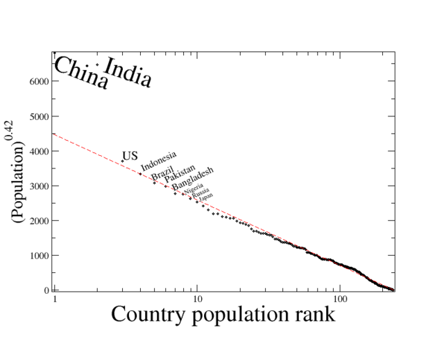
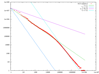
Segments may arise naturally due to actual changes in the behavior of the distribution as rank varies. Most common is the king effect, where the behavior of the top handful of items does not fit the pattern of the rest, as illustrated at the top for country populations, and above for most common words in English Wikipedia. For higher ranks, behavior may change at some point, and be well-modeled by different relations in different regions; on the whole by a piecewise function. For example, if two different power laws fit better in different regions, one can use a broken power law for the overall relation; the word frequency in English Wikipedia (above) also demonstrates this.

The Yule–Simon distribution that results from preferential attachment (intuitively, "the rich get richer" and "success breeds success") simulates a broken power law and has been shown to "very well capture" word frequency versus rank distributions.^[7] It originated from trying to explain the population versus rank in different species. It has also been shown to fit city population versus rank better.^[8]

Rank–size rule

The rank-size rule (or law) describes the remarkable regularity in many phenomena, including the distribution of city sizes, the sizes of businesses, the sizes of particles (such as sand), the lengths of rivers, the frequencies of word usage, and wealth among individuals.

All are real-world observations that follow power laws, such as Zipf's law, the Yule distribution, or the Pareto distribution. If one ranks the population size of cities in a given country or in the entire world and calculates the natural logarithm of the rank and of the city population, the resulting graph will show a linear pattern. This is the rank-size distribution.^[9]

Known exceptions to simple rank–size distributions

While Zipf's law works well in many cases, it tends to not fit the largest cities in many countries; one type of deviation is known as the King effect. A 2002 study found that Zipf's law was rejected in 53 of 73 countries, far more than would be expected based on random chance.^[10] The study also found that variations of the Pareto exponent are better explained by political variables than by economic geography variables like proxies for economies of scale or transportation costs.^[11] A 2004 study showed that Zipf's law did not work well for the five largest cities in six countries.^[12] In the richer countries, the distribution was flatter than predicted. For instance, in the United States, although its largest city, New York City, has more than twice the population of second-place Los Angeles, the two cities' metropolitan areas (also the two largest in the country) are much closer in population. In metropolitan-area population, New York City is only 1.3 times larger than Los Angeles. In other countries, the largest city would dominate much more than expected. For instance, in the Democratic Republic of the Congo, the capital, Kinshasa, is more than eight times larger than the second-largest city, Lubumbashi. When considering the entire distribution of cities, including the smallest ones, the rank-size rule does not hold. Instead, the distribution is log-normal. This follows from Gibrat's law of proportionate growth.

Because exceptions are so easy to find, the function of the rule for analyzing cities today is to compare the city systems in different countries. The rank-size rule is a common standard by which urban primacy is established. A distribution such as that in the United States or China does not exhibit a pattern of primacy, but countries with a dominant "primate city" clearly vary from the rank-size rule in the opposite manner. Therefore, the rule helps to classify national (or regional) city systems according to the degree of dominance exhibited by the largest city. Countries with a primate city, for example, have typically had a colonial history that accounts for that city pattern. If a normal city distribution pattern is expected to follow the rank-size rule (i.e. if the rank-size principle correlates with central place theory), then it suggests that those countries or regions with distributions that do not follow the rule have experienced some conditions that have altered the normal distribution pattern. For example, the presence of multiple regions within large nations such as China and the United States tends to favor a pattern in which more large cities appear than would be predicted by the rule. By contrast, small countries that had been connected (e.g. colonially/economically) to much larger areas will exhibit a distribution in which the largest city is much larger than would fit the rule, compared with the other cities—the excessive size of the city theoretically stems from its connection with a larger system rather than the natural hierarchy that central place theory would predict within that one country or region alone.

See also

• Pareto principle
• Long tail

References

1. Laherrère, J.; Sornette, D. (1998). "Stretched exponential distributions in nature and economy: "fat tails" with characteristic scales". The European Physical Journal B. 2 (4): 525–539. arXiv:cond-mat/9801293. Bibcode:1998EPJB....2..525L. doi:10.1007/s100510050276.
2. "The 200 Largest Cities in the United States by Population 2021". worldpopulationreview.com. Retrieved 2021-03-28.
3. Illustrating the Long Tail, Rand Fishkin, November 24th, 2009
4. Digg that Fat Belly!, Robert Young, Sep. 4, 2006
5. The Long Tail Keyword Optimization Guide - How to Profit from Long Tail Keywords, August 3, 2009, Tom Demers
6. The Small Head, the Medium Body, and the Long Tail .. so, where's Microsoft? Archived 2015-11-17 at the Wayback Machine, 12 Mar 2005, Lawrence Liu's Report from the Inside
7. Lin, Ruokuang; Ma, Qianli D. Y.; Bian, Chunhua (2014). "Scaling laws in human speech, decreasing emergence of new words and a generalized model". arXiv:1412.4846 [cs.CL].
8. Dacey, M F (1 April 1979). "A Growth Process for Zipf's and Yule's City-Size Laws". Environment and Planning A. 11 (4): 361–372. doi:10.1068/a110361. S2CID 122325866.
9. Zipf's Law, or the Rank–Size Distribution Archived 2007-02-13 at the Wayback Machine Steven Brakman, Harry Garretsen, and Charles van Marrewijk
10. "Kwok Tong Soo (2002)" (PDF).
11. Zipf's Law, or the Rank–Size Distribution Archived 2007-03-02 at the Wayback Machine
12. Cuberes, David, The Rise and Decline of Cities, University of Chicago, September 29, 2004,

Further reading

• Brakman, S.; Garretsen, H.; Van Marrewijk, C.; Van Den Berg, M. (1999). "The Return of Zipf: Towards a Further Understanding of the Rank–Size Distribution". Journal of Regional Science. 39 (1): 183–213. doi:10.1111/1467-9787.00129. S2CID 56011475.
• Guérin-Pace, F. (1995). "Rank–Size Distribution and the Process of Urban Growth". Urban Studies. 32 (3): 551–562. doi:10.1080/00420989550012960. S2CID 154660734.
• Reed, W.J. (2001). "The Pareto, Zipf and other power laws". Economics Letters. 74 (1): 15–19. doi:10.1016/S0165-1765(01)00524-9.
• Douglas R. White, Laurent Tambayong, and Nataša Kejžar. 2008. Oscillatory dynamics of city-size distributions in world-historical systems. Globalization as an Evolutionary Process: Modeling Global Change. Ed. by George Modelski, Tessaleno Devezas, and William R. Thompson. London: Routledge. ISBN 978-0-415-77361-4
• The Use of Agent-Based Models in Regional Science—an agent-based simulation study that explains rank–size distribution.

External links

• Media related to Rank-size distribution at Wikimedia Commons