Interquartile range

"IQR" redirects here. For other uses, see IQR (disambiguation).

In descriptive statistics, the interquartile range (IQR) is a measure of statistical dispersion, which is the spread of the data.^[1] The IQR may also be called the midspread, middle 50%, fourth spread, or H‑spread. It is defined as the difference between the 75th and 25th percentiles of the data.^[2][3][4] To calculate the IQR, the data set is divided into quartiles, or four rank-ordered even parts via linear interpolation.^[1] These quartiles are denoted by Q₁ (also called the lower quartile), Q₂ (the median), and Q₃ (also called the upper quartile). The lower quartile corresponds with the 25th percentile and the upper quartile corresponds with the 75th percentile, so IQR = Q₃ −  Q₁^[1]_.

Boxplot (with an interquartile range) and a probability density function (pdf) of a Normal N(0,σ²) Population

The IQR is an example of a trimmed estimator, defined as the 25% trimmed range, which enhances the accuracy of dataset statistics by dropping lower contribution, outlying points.^[5] It is also used as a robust measure of scale^[5] It can be clearly visualized by the box on a box plot.^[1]

Use

Unlike total range, the interquartile range has a breakdown point of 25%^[6] and is thus often preferred to the total range.

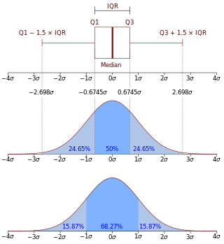
The IQR is used to build box plots, simple graphical representations of a probability distribution.

The IQR is used in businesses as a marker for their income rates.

For a symmetric distribution (where the median equals the midhinge, the average of the first and third quartiles), half the IQR equals the median absolute deviation (MAD).

The median is the corresponding measure of central tendency.

The IQR can be used to identify outliers (see below). The IQR also may indicate the skewness of the dataset.^[1]

The quartile deviation or semi-interquartile range is defined as half the IQR.^[7]

Algorithm

The IQR of a set of values is calculated as the difference between the upper and lower quartiles, Q₃ and Q₁. Each quartile is a median^[8] calculated as follows.

Given an even 2n or odd 2n+1 number of values

first quartile Q₁ = median of the n smallest values

third quartile Q₃ = median of the n largest values^[8]

The second quartile Q₂ is the same as the ordinary median.^[8]

Examples

Data set in a table

The following table has 13 rows, and follows the rules for the odd number of entries.

i	x[i]	Median	Quartile
1	7	Q2=87 (median of whole table)	Q1=31 (median of lower half, from row 1 to 6)
2	7
3	31
4	31
5	47
6	75
7	87
8	115		Q3=119 (median of upper half, from row 8 to 13)
9	116
10	119
11	119
12	155
13	177

For the data in this table the interquartile range is IQR = Q₃ − Q₁ = 119 - 31 = 88.

Data set in a plain-text box plot

                             +−−−−−+−+
               * |−−−−−−−−−−−|     | |−−−−−−−−−−−|
                             +−−−−−+−+

 +−−−+−−−+−−−+−−−+−−−+−−−+−−−+−−−+−−−+−−−+−−−+−−−+   Number line
 0   1   2   3   4   5   6   7   8   9   10  11  12

For the data set in this box plot:

• Lower (first) quartile Q₁ = 7
• Median (second quartile) Q₂ = 8.5
• Upper (third) quartile Q₃ = 9
• Interquartile range, IQR = Q₃ - Q₁ = 2
• Lower 1.5*IQR whisker = Q₁ - 1.5 * IQR = 7 - 3 = 4. (If there is no data point at 4, then the lowest point greater than 4.)
• Upper 1.5*IQR whisker = Q₃ + 1.5 * IQR = 9 + 3 = 12. (If there is no data point at 12, then the highest point less than 12.)
• Pattern of latter two bullet points: If there are no data points at the true quartiles, use data points slightly "inland" (closer to the median) from the actual quartiles.

This means the 1.5*IQR whiskers can be uneven in lengths. The median, minimum, maximum, and the first and third quartile constitute the Five-number summary.^[9]

Distributions

The interquartile range of a continuous distribution can be calculated by integrating the probability density function (which yields the cumulative distribution function—any other means of calculating the CDF will also work). The lower quartile, Q₁, is a number such that integral of the PDF from -∞ to Q₁ equals 0.25, while the upper quartile, Q₃, is such a number that the integral from -∞ to Q₃ equals 0.75; in terms of the CDF, the quartiles can be defined as follows:

${\displaystyle Q_{1}={\text{CDF}}^{-1}(0.25),}$

${\displaystyle Q_{3}={\text{CDF}}^{-1}(0.75),}$

where CDF⁻¹ is the quantile function.

The interquartile range and median of some common distributions are shown below

Distribution	Median	IQR
Normal	μ	2 Φ−1(0.75)σ ≈ 1.349σ ≈ (27/20)σ
Laplace	μ	2b ln(2) ≈ 1.386b
Cauchy	μ	2γ

Interquartile range test for normality of distribution

The IQR, mean, and standard deviation of a population P can be used in a simple test of whether or not P is normally distributed, or Gaussian. If P is normally distributed, then the standard score of the first quartile, z₁, is −0.67, and the standard score of the third quartile, z₃, is +0.67. Given mean = ${\displaystyle {\bar {P}}}$ and standard deviation = σ for P, if P is normally distributed, the first quartile

${\displaystyle Q_{1}=(\sigma \,z_{1})+{\bar {P}}}$

and the third quartile

${\displaystyle Q_{3}=(\sigma \,z_{3})+{\bar {P}}}$

If the actual values of the first or third quartiles differ substantially^{[clarification needed]} from the calculated values, P is not normally distributed. However, a normal distribution can be trivially perturbed to maintain its Q1 and Q2 std. scores at 0.67 and −0.67 and not be normally distributed (so the above test would produce a false positive). A better test of normality, such as Q–Q plot would be indicated here.

Outliers

Box-and-whisker plot with four mild outliers and one extreme outlier. In this chart, outliers are defined as mild above Q3 + 1.5 IQR and extreme above Q3 + 3 IQR.

The interquartile range is often used to find outliers in data. Outliers here are defined as observations that fall below Q1 − 1.5 IQR or above Q3 + 1.5 IQR. In a boxplot, the highest and lowest occurring value within this limit are indicated by whiskers of the box (frequently with an additional bar at the end of the whisker) and any outliers as individual points.

See also

• Interdecile range – Statistical measure
• Midhinge – average of the first and third quartilesPages displaying wikidata descriptions as a fallback
• Probable error – Measure of statistical dispersion
• Robust measures of scale – Statistical indicators of the deviation of a sample

References

1. Dekking, Frederik Michel; Kraaikamp, Cornelis; Lopuhaä, Hen Paul; Meester, Ludolf Erwin (2005). A Modern Introduction to Probability and Statistics. Springer Texts in Statistics. London: Springer London. doi:10.1007/1-84628-168-7. ISBN 978-1-85233-896-1.
2. Upton, Graham; Cook, Ian (1996). Understanding Statistics. Oxford University Press. p. 55. ISBN 0-19-914391-9.
3. Zwillinger, D., Kokoska, S. (2000) CRC Standard Probability and Statistics Tables and Formulae, CRC Press. ISBN 1-58488-059-7 page 18.
4. Ross, Sheldon (2010). Introductory Statistics. Burlington, MA: Elsevier. pp. 103–104. ISBN 978-0-12-374388-6.
5. Kaltenbach, Hans-Michael (2012). A concise guide to statistics. Heidelberg: Springer. ISBN 978-3-642-23502-3. OCLC 763157853.
6. Rousseeuw, Peter J.; Croux, Christophe (1992). Y. Dodge (ed.). "Explicit Scale Estimators with High Breakdown Point" (PDF). L1-Statistical Analysis and Related Methods. Amsterdam: North-Holland. pp. 77–92.
7. Yule, G. Udny (1911). An Introduction to the Theory of Statistics. Charles Griffin and Company. pp. 147–148.
8. Bertil., Westergren (1988). Beta [beta] mathematics handbook : concepts, theorems, methods, algorithms, formulas, graphs, tables. Studentlitteratur. p. 348. ISBN 9144250517. OCLC 18454776.
9. Dekking, Kraaikamp, Lopuhaä & Meester, pp. 235–237

External links

• Media related to Interquartile range at Wikimedia Commons